Working Principle of OCT
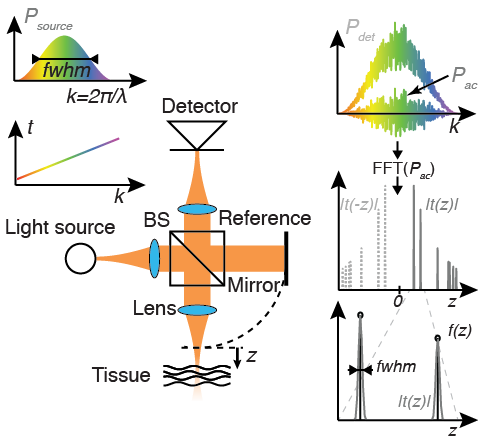
Basic OCT setup, with a beam splitter (BS) separating the light into the sample arm towards the tissue, and the reference arm towards the mirror, respectively. The plots display the source spectrum as well as the resulting interference pattern, and illustrate the reconstruction process. The tomogram  broadens the discrete reflections in the reflection profile
  to a full width at half maximum (fwhm) characteristic of the OCT system.
Frequency domain signal
OCT measures the subsurface microstructure of biological tissue by discerning light reflected from different depths within the sample. Similar to ultrasound imaging, the signal from a deeper-lying structure has traveled a longer distance and reaches the detector with a delay. The speed of sound is sufficiently low to directly record the delay between the various echoes from the sample. In contrast, light travels at much greater speed that precludes direct detection of the delay. Instead, OCT employs interferometric detection and compares the signal reflected from the sample with a static reference signal. Fig. 1 displays the basic configuration of an OCT instrument. Light from a source covering a wide wavelength spectrum is separated by a beam splitter into a reference and a sample arm. Biological tissue is partially transparent at the employed wavelength range in the near infrared. Accordingly, the probing light propagates through the sample tissue, and is scattered and reflected by internal structure at different depths. Part of this backscattered light will reach the detector where it interferes with the light from the reference arm that was simply reflected by a mirror. The interference signal is converted by the detector into an electrical signal and is of the form

where  and
and  are proportional to the electromagnetic field reflected in the reference and the sample arm, respectively, and the star indicates the complex conjugate. Of interest here are the last two interference terms.
Optical Frequency Domain Imaging (OFDI) and other swept source implementations of OCT use a wavelength-swept laser source that sweeps a broad wavelength range in a short time. The interference signal, recorded as a function of time, corresponds to the signal as a function of the wavenumber  , where
  is the wavelength. Alternatively, camera-based spectral domain OCT systems employ broad band light and a spectrometer to record an equivalent signal. The first interference term in the above equation can be expressed as

where is the sample reflectivity profile as a function of  , the depth position inside the sample relative to the reference arm length. The factor 2 takes into account the double pass from the source to the sample and back from the sample towards the detector.
  is the spectral shape of the source spectrum, and
  .
.
Recording the signal as a function of the wavenumber is equivalent to taking the Fourier transform of the axial reflectivity profile. Accordingly, inverse Fourier transformation of the recorded signal will reconstruct the tomogram of the sample reflectivity profile:

The Fourier transformation connects the spatial domain () with the spatial frequency or wavenumber domain  . The reconstructed amplitude
  is proportional to the amplitude of the electromagnetic field and
  to the intensity scattered in the sample at depth . Tomograms are displayed in logarithmic scale:

The recorded fringe signal contains two complex conjugate interference terms, which result in a mirror symmetry in the reconstructed tomogram. If the first term creates the tomogram , then the second term produces the tomogram  , mirrored about the zero differential path length. Generally, this results in a disturbing overlap that can be avoided by adjusting sufficient path length difference between the reference and the sample arm, or by employing additional strategies to separate the two terms.
Although the reconstructed tomogram is a close image of the original structure, the spectral shape of the source effectively performs a weighting of the spatial frequency spectrum. Only the range of spatial frequencies covered by the employed light source is accessible. As a result, the reconstructed signal is a filtered image of the original structure, expressed by the convolution of the original reflectivity profile with the point spread function (PSF) of the OCT system. This PSF is equivalent to the inverse Fourier transform of the spectral shape function  . The tomogram can be expressed as

with the star symbol indicating the convolution operator.  is the coherence function of a light source with the power spectral density , explaining the origin of the term ‘optical coherence tomography’.
A single reflector in the original sample reflectivity function results in a peak of a finite width in the reconstructed tomogram. Assuming a source spectrum with a Gaussian shape, the full width at half maximum (fwhm) of the spectrum as a function of wavenumber  is related to the fwhm of the peak
  in the reconstructed tomogram by

The wider the spectrum covered by the light source, the better the structure of the axial tomogram is resolved.
Imaging lateral structure
In order to resolve structure in the lateral direction, the probe beam is focused into a narrow beam. It is then scanned in the lateral direction while constantly acquiring depth profiles, by means of galvanometric mirrors. At each scan location, the axial depth profile is acquired by recording one interference spectrum. Assembling all depth profiles of a lateral scan results in a cross-sectional image. Acquiring multiple cross-sectional images while scanning along the remaining spatial coordinate enables volumetric imaging.
For endoscopic and probe-based imaging of luminal organs, the natural way to scan a spot over the cylindrical inner surface of the organ is by rotating a side-looking imaging probe inside a protective sheath placed in the center of the lumen. The depth profiles measured during one rotation of the probe can then be mapped into Cartesian coordinates to provide a cross-sectional view of the lumen wall. Combined pull-back motion of the probe inside the sheath defines a helical scan pattern on the lumen surface and enables volumetric imaging of entire segments of the organ.
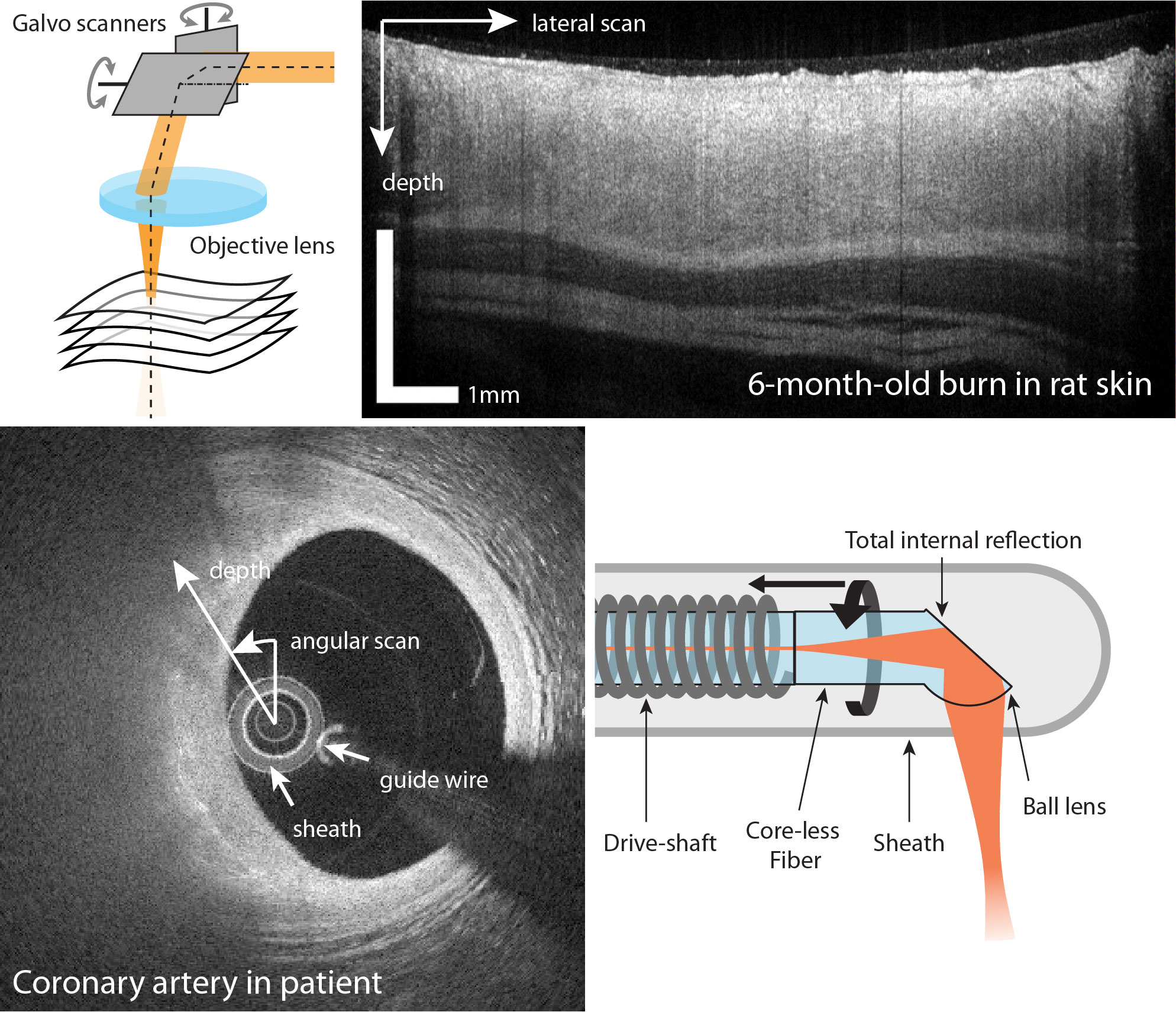
Lateral structure is resolved by scanning a focused beam over the sample. This can be achieved in a ‘bench-top’ setting with galvanometric mirrors, or with fiber-based imaging probes in a catheter configuration.
Adapted from [Villiger, M. L. & Bouma, B. E. Physics of Cardiovascular OCT